Introduction

With the apparition of internet, a large amount of data have been generated. In fact, this a exponential growth. For example, each day about 500M tweets are sent, 95M photos and videos are shared in Instagram, 500M photos are been uploaded. This exponential growth has allowed the use of new techniques in Artificial Intelligence. For example Deep Learning, where models can use this large amount of data to create useful applications, which we use everyday. In this dynamic interaction, where models and data combine into services, we need to address an important aspect: privacy. Privacy is an important area which is presented in many branches of science. It is an important property, which must be maintained. However, this can be different, according to the context in which is applied. In particular case of deep learning, we are interested in preserve privacy at both levels:

1. Data, we need to assure, that the data been used, must retain its privacy property, and in
2. Models, we must protect the learned information, such as, no leaking is present.
   In the following sections, we will apply different privacy techniques in both levels.

Differential Privacy (DP)

Suppose we have a large data set, for which we have little or no labels. In a case like this, we could apply different techniques to label the data. Among them, we could use external models to classify our data. Then, we can average their predictions (similar to voting models) and get our labels. Of course, we need to train our own model afterwards. However, how can we guarantee that no information from the external data set will be leaked into our labels. At first, it could seem innocent to think that, we cannot use the external models to get information about their data sets. In truth, it can be done. Therefore, we need to implement a framework, which:

1. Allow to label our data, and at the same time.
2. Maintains the privacy of the external data sets.

The DP framework is the answer to this problem. DP, allow us to use the predictive capacity of external models, in a fashion, where privacy is maintained. In fact, we add a new hyperparameter to our training, which will maintain the privacy. In this scenario, a set of teachers (external models) will be used to aid in the generation of labels. In this setting, we use each teacher prediction to get a label.

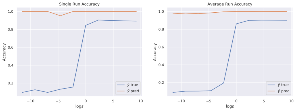
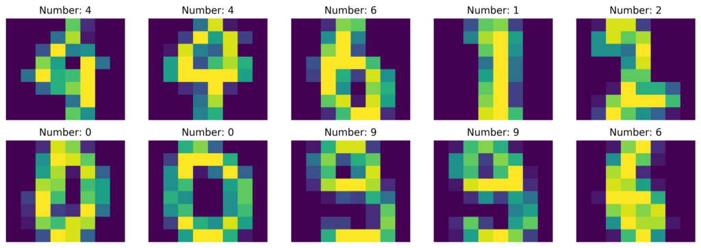
Then, we can take the maximum in a voting fashion. However, we need to take into consideration the privacy factor. Therefore, we will add an extra factor into the process. This, will be defined as epsilon, and will measure the level of information leaking as well the and the maintained privacy. Thus, epsilon became another hyperparameter that we must tune. Furthermore, this hyperparameter, will ensure that no information is leaking into the generated labels. Now, since we will add noise, there are many approaches we can use to generate it. Some famous options are Gaussian and Laplace noise. Now, let’s explore DP with an example. In this example, we are going to use the digits data set. This data set, as we can see in the image; contains handwritten digits, which vary from zero to nine. The images are contained into an array.

Now, we need to simulate the teachers, remember that these teachers will help us to generated our labels. In this case, they can be represented by any model. For simplicity, lets assume that we already have ten teachers. This means, we have already divided the data into eleven blocks. Ten for the teachers and one for our local model. In this setting is important to add randomness to the split process. In real applications however, ten teachers could result in no variations when applying PATE analysis (more later), but for now it will be enough for our purposes. Using the teachers, we will obtain a set of different predictions to our local data set as seen below:

array([[1., 6., 6., ..., 6., 6., 6.],
       [1., 9., 9., ..., 9., 9., 9.],
       [1., 9., 9., ..., 9., 9., 9.],
       ...,
       [1., 6., 6., ..., 6., 6., 6.],
       [1., 8., 2., ..., 2., 8., 9.],
       [1., 3., 3., ..., 3., 3., 3.]])

Now, we need to add the privacy factor: epsilon into the label generation. For this, we will use the Laplacian noise as follows:

def laplacian_noise(preds, epsilon = 0.1):
    new_labels = list()
    for pred in preds:
        label_count = np.bincount(pred.astype(int), minlength = 10)
        beta = 1/epsilon
        for i in range(len(label_count)):
            label_count[i] += np.random.laplace(0, beta, 1)
        new_label = np.argmax(label_count)
        new_labels.append(new_label)
    return new_labels

In this case, since we have ten classes, the bincount function takes a value of 10. At this stage, we already have our labels, the next step is training our local model. For that, lets use the following shallow network:

class Net(nn.Module):
    def __init__(self):
        super().__init__()
        self.fc1 = nn.Linear(64, 50)
        self.fc2 = nn.Linear(50, 50)
        self.output = nn.Linear(50, 10)

    def forward(self, x):
        x = F.relu(self.fc1(x))
        x = F.relu(self.fc2(x))
        x = F.log_softmax(self.output(x), dim = 1)
        return x

Now, lets explore the effect of the epsilon hyperparameter in more detail. Since we are using it to preserve privacy, it is important to note that:

• Larger values will result in more privacy leaking, but high accuracy and,
• Lower values will result in less privacy leaking, but low accuracy.

To see this, lets repeat the process, and generate labels using different epsilon values from 1e-5 to 10e+3. Also, lets repeat the training process. Finally, lets compare the accuracy result using the generated labels against the real ones. As we can see in the figure, there is a trade-off between privacy and accuracy.