Visualization of Learning Representations with PCA and UMAP

Deep learning models, such as neural networks, build abstract representations of data during the training phase. In this stage, the goal is to optimize a cost function—either by minimizing or maximizing it—using algorithms like those from the gradient descent family.

In neural networks, this process is applied to each layer of the model. Thus, each layer learns a specific representation of the data. Since the layers are interconnected, a hierarchical structure is formed: deeper layers—those closer to the output—capture complex patterns generated by the preceding layers.

A particularly interesting aspect is understanding how information is structured in these deep layers. This is an active area of research, as deep neural networks are often treated as black boxes.

During the development of our master’s thesis in Data Science, we faced this challenge. We designed a deep learning model that combined image and time series data, using a convolutional network and a temporal convolutional network. This model was applied to a binary classification problem.

To analyze how the progressive incorporation of information influenced the model’s decision-making, we selected a variable of interest called $\text{Seq}$, distributed across five columns: $\text{Seq}_1, \text{Seq}_2, \ldots, \text{Seq}_5$.

We selected a representative sample from both classes and fed it into the model, recording the activations generated in the penultimate layer for each iteration, as the $\text{Seq}_i$ variables were progressively added.

This allowed us to construct an activation matrix:

$$
M \in \mathbb{R}^{m \times n}
$$

where $m$ represents the number of selected samples and $n$ the number of neurons in the penultimate layer.

Since $M$ is high-dimensional, it was necessary to apply dimensionality reduction techniques to visualize the learned representations. The goal was to project $M$into a new space of dimension $k$, such that $k < n $:

$$
M’ = f(M), \quad M’ \in \mathbb{R}^{m \times k}
$$

For this task, we used two widely known algorithms:

Principal Component Analysis (PCA)

PCA transforms the data using orthogonal linear combinations that maximize variance. Mathematically, it seeks a projection matrix $W$ such that:

$$
M’ = M W
$$

where the columns of $W$ are the eigenvectors of the covariance matrix of $M$, associated with the largest eigenvalues.

Uniform Manifold Approximation and Projection (UMAP)

UMAP is a nonlinear technique that preserves both the local and global structure of the data. Unlike PCA, UMAP constructs a proximity graph in the high-dimensional space and projects it into a lower-dimensional space, optimizing the preservation of topology. Although its mathematical formulation is more complex, it is based on minimizing the divergence between probability distributions in both spaces.

Visualization

For visualization, we chose a reduced space of dimension $k = 2$. We iterated incrementally through the variables $\text{Seq}_1$ to $\text{Seq}_5$ capturing the corresponding activations at each step.

The results obtained using PCA are shown below:

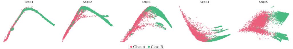
As can be observed, as the number of variables increases, the separation between classes becomes more evident. Additionally, the structure of the class space progressively transforms, with $\text{Seq}_5$ showing a clearer and more distinguishable separation between classes.

This behavior is also evident when applying UMAP:

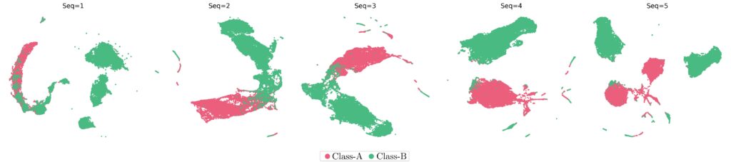
In these visualizations, it is clear how the classes separate more distinctly as more information from the $\text{Seq}$ variable is incorporated. Comparing both techniques, we noticed that the model improves its ability to differentiate between classes as the input data becomes richer.

Having two visualization approaches allows us to evaluate the relevance of the $\text{Seq}$ variable from complementary perspectives: PCA offers a linear and global view, while UMAP provides a nonlinear perspective that preserves local topology.

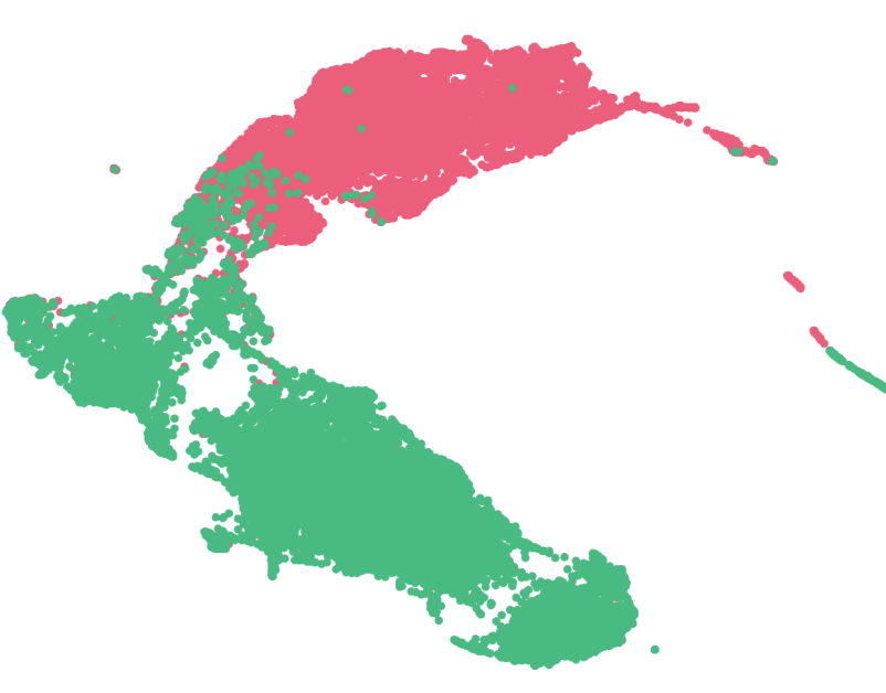
Finally, to more dynamically observe how the representation space transforms, we decided to create an animation using the visualizations obtained with UMAP. The result is shown below:

Conclusions

This study allowed us to explore how the internal representations of a deep learning model evolve as relevant information is progressively incorporated. Through dimensionality reduction techniques like PCA and UMAP, we were able to visualize how the class space is structured in the model’s penultimate layer.

The results show that:

Incrementally adding variables improves class differentiation.
PCA and UMAP offer complementary perspectives for analyzing data structure.
The $\text{Seq}$ variable has a significant impact on the model’s ability to discriminate between classes.

These visualizations not only enrich the technical analysis but also contribute to the interpretability of models that are traditionally considered black boxes. In future research, this approach could be extended to other types of variables and architectures, contributing to a deeper understanding of representational learning in neural networks.